• Home
• Data
• Cap Vol

Cap Vol

FinPricing offers:

Four user interfaces:

View:

Interest Rate Cap Implied Volatility Surface Construction Guide

An implied volatility is the volatility implied by the market price of an option based on the Black-Scholes  option pricing model. In cap market, a cap or floor is quoted by implied volatilities but not prices. An interest rate cap volatility surface is a three-dimensional plot of the implied volatility of a cap as a function of strike and maturity.

The term structures of implied volatilities provide indications of the market’s near- and long-term uncertainty about future short- and long-term forward rates. A crucial property of the implied volatility surface is the absence of arbitrage.

When the implied volatilities are plotted against the strike price at a fixed maturity, one often observes a skew or smile pattern, which has been shown to be directly related to the conditional non-normality of the underlying return risk-neutral distribution. In particular, a smile reflects fat tails in the return distribution whereas a skew indicates return distribution asymmetry. Furthermore, how the implied volatility smile varies across option maturity and calendar time reveals how the conditional return distribution non-normality varies across different conditioning horizons and over different time periods.

The pricing accuracy and pricing performance of option models crucially depends on absence of arbitrage in the implied volatility surface: an input implied volatility surface that is not arbitrage-free invariably results in negative transition probabilities and/ or negative volatilities, and ultimately, into mispricings.

To construct a reliable volatility surface, it is necessarily to apply robust interpolation methods to a set of discrete volatility data. Arbitrage free conditions may be implicitly or explicitly embedded in the procedure. Typical approaches are

• Local Volatility Model: a generalization of the Black-Scholes model.
• Stochastic Volatility Models: such as SABR, Heston, Levy.
• Parametric or Semi-Parametric Models: such as SVI model, Omega model, etc.
• Market Volatility Model: directly modeling the implied volatility dynamics
• Interpolation/Extrapolation Model: interpolating or extrapolating volatility data using specific function forms.

At FinPricing, we use the SABR model to construct cap implied volatility surfaces following the best market practice.

Any volatility models must meet arbitrage free conditions. Typical arbitrage free conditions are

• Static arbitrage free condition: Static arbitrage free condition makes it impossible to invest nothing today and receive positive return tomorrow.
• Calendar arbitrage free condition: The cost of a calendar spread should be positive.
• Vertical (spread) arbitrage free condition: The cost of a vertical spread should be positive.
• Horizontal (butterfly) arbitrage free condition: The cost of a butterfly spread should be positive.

Vertical arbitrage free and horizontal arbitrage free conditions for volatility surfaces depend on different strikes. There is no calendar arbitrage in cap volatility surfaces as caps with different maturities have different cash flows and are associated with different indices. In other words, they can be treated independently.

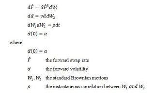
SABR stands for “stochastic alpha, beta, rho” referring to the parameters of the model. The SABR model is a stochastic volatility model for the evolution of the forward price of an asset, which attempts to capture the volatility smile/skew in derivative markets.

There is a closed-form approximation of the implied volatility of the SABR model. In the cap volatility case, the underlying asset is the forward interest rate. The dynamics of the SABR model.

• α is the volatility that is tied closely to the at-the-money volatility value.
• β is the exponent that is related to the backbone that the ATM volatility traces when the ATM forward rate varies.
• ρ is the correlation that describes the “skew” or average slope of the volatility curve across strike.
• υ is the volatility of volatility that describes the “smile” or curvature/convexity of the volatility curve across the strike for a given term and tenor.

For each term (expiry) and tenor of the cap, conduct the following calibration procedure.

• The β parameter is estimated first and typically chosen a priori according to how the market prices are to be observed.
• Alternatively β can be estimated by a linear regression on a time series of ATM volatilities and of forward rates.
• After β is set, we can obtain α by using σ_ATM to solve the following equation
• The Viete method is used to solve this equation.
• Given the α,β solved above, we can find the optimized value of (ρ,v) by minimizing the distance between the SABR model output volatilities and market volatilities across all strikes for each term and tenor.
• The Levenberg-Marquardt least-squares optimization routine is used for optimization.
• After (α, β, ρ, υ) calibrated, one can generate SABR volatility (cap volatility) for any moneyness.

Repeat the above process for each term and tenor.

• Swap rate curves
• SOFR curves
• OIS curves
• interest rate curves
• Inflation swap rate curves
• Forward yield curves
• FX forward curve
• FX vol surface