Bermudan Swaption
FinPricing offers:
Four user interfaces:
- Data API.
- Excel Add-ins.
- Model Analytic API.
- GUI APP.

Interest rate Bermudan swaptions give the holders the right but not the obligation to enter an
interest rate swap at predefined dates.
| 1. Bermudan Swaption Introduction |
A interest rate Bermudan swaption is one of the fundamental ways for an investor to enter a
swap. Comparing to regular swaptions, Bermudan swaptions
provide market participants more flexibility and control over the exercising of an option and less restriction.
Given those flexibilities, a Bermudan swaption is more expensive than a regular
European swaption. In terms of valuation, it is also much more complex.
| 2. Bermudan Swaption Payoffs |
At the maturity T, the payoff of a Bermudan swaption is given by
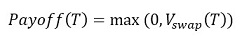
where V_swap (T) is the value of the underlying swap at T
At any exercise date T_i, the payoff of the Bermudan swaption is given by
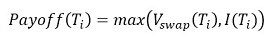
Where V_swap (T_i) is the exercise value of the Bermudan swap and I(T_i) is the intrinsic value.
| 3. Valuation Model Selection Criteria |
Given the complexity of Bermudan swaption valuation, there is no closed form solution. Therefore, we need to select
an interest rate term structure model and a numeric solution to price Bermudan swaptions.
Popular IR term structure models in the market are Hull-White, Linear Gaussian Model (LGM), Quadratic Gaussian Model (QGM),
Heath Jarrow Morton (HJM), Libor Market Model (LMM). HJM and LMM are too complex while Hull-White is inaccurate for
computing sensitivities. Therefore, we choose either LGM or QGM.
After selecting a term structure model, we need to choose a numeric approach to approximate the underlying
stochastic process of the model. Commonly used numeric approaches are tree, partial differential equation (PDE),
lattice, and Monte Carlo simulation. Tree and Monte Carlo are notorious for inaccuracy in sensitivity calculation.
Therefore, we choose either PDE or lattice. Our final decision is to use LGM plus lattice.
| 4. LGM Model |
The dynamics is expressed as
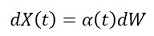
2here X is the single state variable; W is the Wiener process.
The numeraire is given by

| 5. LGM Assumptions and Calibration |
The LGM model is mathematically equivalent to the Hull-White model but offers significant improvements in calibration
stability and accuracy. It is also more accurate and stable in sensitivity calculation. The state variable is normally
distributed under the appropriate measure. The LGM model has only one stochastic driver (one-factor), thus changes in
rates are perfected correlated.
At time t, X(0)=0 and H(0)=0. Thus Z(0,0;T)=D(T). In other words, the LGM automatically fits today’s
discount curve or yield curve. To calibrate
swaption implied volatilities, first select a group of market
swaptions and then solve parameters by minimizing the relative error between the market
swaption prices and the LGM model
swaption prices.
| 6. Valuation Practical Guide |
| References |